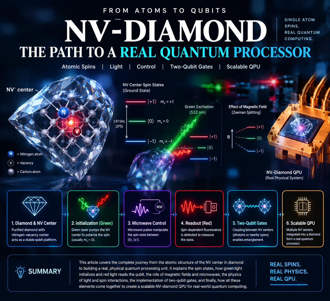
A journey from the atomic structure of an NV center to initialization, microwave control, optical readout, ODMR, and eventually a physical quantum processor

C — C — C
|   |   |
C — C — C
|   |   |
C — C — C

Of course, the real structure is three-dimensional.

The important point is that the diamond lattice is normally very regular.

But sometimes one carbon atom is replaced by a different atom, or one position in the lattice is empty.

These imperfections are called defects or color centers.

One particularly important defect is the NV center.

3. What Is an NV Center?

NV stands for:

N = Nitrogen

V = Vacancy

An NV center consists essentially of:

one nitrogen atom replacing a carbon atom

an adjacent missing carbon atom, called a vacancy

Conceptually:

      C
      |
C — N — [Vacancy]
      |
      C

The actual atomic geometry is three-dimensional, but this picture gives the basic idea.

The nitrogen and vacancy together create a special electronic environment inside the diamond.

The axis connecting the nitrogen and vacancy is called the NV axis.

There are four equivalent NV orientations in a diamond crystal

4. What Does NV⁻ Mean?

You will frequently see:

NV⁻

The − means the NV center is in a negative charge state.

There are different charge states of NV centers, but the negatively charged NV⁻ center is the one most commonly used for quantum sensing and quantum information experiments.

For our discussion, when we say "NV center," we will generally mean:

NV⁻

5. Where Does the Qubit Come From?

Now we reach the most important idea.

The NV⁻ center has an electronic spin.

Its ground electronic state behaves as a spin-1 system.

We write:

S=1 

This does not mean that an electron is literally spinning like a tiny ball.

"Spin" is an intrinsic quantum property of particles.

6. What Does S = 1 Mean?

For a spin quantum number S, the possible spin projections are:

m_s = -S,...,0,...,+S

For:

S = 1

we therefore get:

m_s = -1, 0, +1

So the NV ground-state spin has three possible spin projections:

          ms = +1
             |
             |
          ms = 0
             |
             |
          ms = -1

This is an important distinction : S

describes the total spin quantum number : m_s

describes the spin projection along a chosen axis.

So:

possible ms:

+1
 0
-1

7. But a Qubit Has Only Two States

You might immediately notice a problem.

A normal qubit has two computational states:

∣0⟩

and

∣1⟩

But the NV electron spin has three states:

m_s = 0, +1, -1 

So the NV electron spin is technically a qutrit-like three-level system, not directly a two-level qubit.

For quantum computing, we normally select two of those states.

For example:

∣0⟩ = ms ​=  0 

and

∣1⟩ = ms = −1

The m_s = +1 state can be treated as another available level but excluded from the chosen computational basis.

Therefore:

ms = +1     ← unused/extra level
            


ms = 0      ← |0⟩
              |
              |  qubit
              |
ms = -1     ← |1⟩

This is how a physical NV spin can provide a qubit.

8. The Natural Energy Levels

At zero external magnetic field, the three ground-state spin levels are not all at the same energy.

The m_s = 0 state is lower.

The m_s = +1 and m_s = -1 states are approximately degenerate, meaning they have the same energy.

The energy separation between m_s = 0 and m_s = 1 is approximately:

D ≈ 2.87 GHz

This is called the zero-field splitting.

Conceptually:

ms = +1  ─────────
              ↑
              │  2.87 GHz
              ↓
ms =  0  ─────────

ms = -1  ─────────

At zero magnetic field:

E+1 ≈ E−1​

9. Why Is 2.87 GHz Important?

This number becomes extremely important later.

A difference of approximately 2.87 GHz corresponds to microwave-frequency energy.

Therefore, if we want to manipulate the NV spin, we can apply a microwave field near the appropriate frequency.

In simple terms:

The energy gap determines the microwave frequency required to drive the spin transition.

This is the foundation of microwave control.

10. What Happens When We Shine Green Light?

Now we introduce the first major experimental tool:

Green laser

A commonly used excitation wavelength is approximately:

532 nm

The green laser primarily provides optical excitation.

It gives the NV center enough energy to move from its electronic ground state to an electronically excited state.

Very simplified:

        Excited electronic state
                 ↑
                 │
            GREEN LIGHT
                 │
                 │
        Ground electronic state

So:

Green light → electronic excitation

But something much more interesting happens during the subsequent relaxation.

11 Green Light Does Not Directly Mean "Spin Becomes  0"

This is an important correction to a common oversimplification.

It is tempting to say:

"Green laser changes m_s = 1 into m_s = 0"

That is not the best description.

The green photon primarily causes optical excitation.

The spin polarization toward  m_s = 0 happens because of the different relaxation pathways available to the spin states.

This distinction is important if you want to build the actual experiment.

12. The NV Relaxation Process

After optical excitation, the NV can return toward the ground state through different pathways.

The simplified picture is:

                    Green photon
                         ↓
                  Excited state
                   /          \
                  /            \
                 ↓              ↓
          Fluorescence       Intersystem
             pathway          crossing
                 ↓              ↓
          Ground state       Singlet state
                                ↓
                                ↓
                         Ground-state m_s=0

The second pathway involves what is called intersystem crossing (ISC) through metastable singlet states.

The important practical result is:

Population in ms​ = ±1 is preferentially redirected toward m_s = 0

Repeated optical excitation cycles therefore polarize the spin toward m_s = 0

This process is called: 

Optical spin initialization or Optical pumping

13. What Does "Initialization" Mean?

Initialization simply means:

Put the quantum system into a known starting state.

For example: ∣0⟩=ms​=0

Green optical pumping can therefore be used to approximately prepare: ∣0⟩

before a quantum experiment begins.

Unknown state
     ↓
Green laser
     ↓
Optical pumping
     ↓
Mostly ms = 0
     ↓
Known starting state

This is extremely useful for quantum computing.

A quantum computer cannot reliably execute a quantum algorithm if we don't know the initial state.

14. Where Does the Red Light Come From?

Now we can understand the fluorescence.

After the NV is optically excited, it can return toward the ground state while emitting photons.

The NV fluorescence has a broad spectrum extending through the red region, with a characteristic zero-phonon line around 637 nm.

The simplified experimental picture is:

532 nm green
      ↓
    NV⁻
      ↓
electronic excitation
      ↓
relaxation
      ↓
red fluorescence

Therefore:

Green = excitation

Red fluorescence = optical emission during relaxation.

15. Why Is the Red Fluorescence Important?

Because the brightness depends on the spin state.

This gives us something extremely valuable:

We can indirectly measure the spin using light.

The NV does not simply produce exactly the same fluorescence for every spin state.

The m_s = 0 state generally produces stronger fluorescence than ms​ = ±1,

 because the latter have a greater probability of taking the non-radiative intersystem-crossing pathway.

So approximately: ms = 0

Green → NV → strong fluorescence
                  █████████


ms = ±1

Green → NV → weaker fluorescence
                  ██████

The exact brightness difference depends on the experimental conditions.

16. This Gives Us Optical Spin Readout

Now we have another essential ingredient of a qubit.

We can:

prepare the spin,

manipulate the spin,

measure the spin.

The measurement is indirect

Spin state
    ↓
Different optical pathway
    ↓
Different fluorescence brightness
    ↓
Photon detector
    ↓
Measurement

This is called optical spin readout.

17. The Microwave Comes In

Now suppose we have initialized the NV into: ms ​= 0

A microwave source can generate an electromagnetic field near this frequency.

When its frequency matches the energy difference between the spin states, the NV can respond strongly.

This is called: Resonance

18. What Is Resonance?

Imagine pushing a swing.

If you push randomly:

push... wait... push... wait...

you don't efficiently increase the swing's motion.

But if you push at the correct rhythm:

push → push → push → push

the swing responds strongly.

The same basic idea applies to the spin.

If: hν ≈ ΔE

then the microwave frequency matches the energy difference.

The spin transition can therefore be driven efficiently.

19. Microwave Does Not Simply "Reduce Energy"

Another important correction:

A microwave is not simply a tool for "reducing the energy" of the NV.

Instead, the microwave field drives transitions between quantum states.

For example:

ms ​= 0 ↔ ms ​= −1   or   ms ​= 0 ↔ ms ​= + 1

depending on the chosen frequency and experimental conditions.

So the better mental model is:

Microwave = controlled spin manipulation

20. The Complete Basic Cycle

Now we can combine everything.

Step 1 — Initialize

Use green light:  Green → optical pumping → ms ​= 0

Step 2 — Manipulate

Apply microwave radiation: ms​ = 0 → ms​ = ± 1

or create a quantum superposition.

Step 3 — Read

Apply green light again.

The NV fluoresces differently depending on the spin state.

Step 4 — Detect

Measure the emitted photons.

So:

       GREEN
         ↓
   ┌───────────┐
   │ Initialize│
   └─────┬─────┘
         ↓
      ms = 0
         ↓
    MICROWAVE
         ↓
 Spin manipulation
         ↓
       GREEN
         ↓
  Fluorescence
         ↓
 Photon detector
         ↓
     Readout

This is the basic operating principle behind NV spin experiments.

21. What Happens If We Start at m_s = ±1?

Suppose the NV starts in: ms ​= −1

We apply green light.

The NV becomes optically excited.

During relaxation, the spin-dependent pathways preferentially return population toward: ms ​= 0

After repeated optical cycles, the population becomes strongly biased toward m_s = 0

So:

ms = -1
   ↓
Green excitation
   ↓
Relaxation / ISC
   ↓
Preferential return
   ↓
ms = 0

It is preferential, not perfectly deterministic.

22. Now Introduce the Magnetic Field

So far we have considered approximately zero magnetic field.

Now apply an external magnetic field.

A magnetic field interacts with the electron spin through the Zeeman effect.

The most important consequence for us is:

The m_s = +1 and m_s = -1 states split in energy.

Without magnetic field:

ms = +1 ─────────
         
ms = -1 ─────────

With magnetic field:

ms = +1 ─────────────

ms =  0 ─────────

ms = -1 ───────

The exact energies depend on the field magnitude and direction.

23. Does the Magnetic Field Flip the Spin?

No—not automatically.

This is another important distinction.

A static magnetic field primarily changes the energy levels.

It does not simply say:

"The spin is now +1."

Instead:

Magnetic field
      ↓
Energy levels change
      ↓
Transition frequency changes
      ↓
Microwave frequency can be selected
      ↓
Microwave drives the desired transition

So the magnetic field gives us a way to control and distinguish the spin transitions.

24. The Simplified Hamiltonian

Once you understand the physical picture, we can express it mathematically.

A simplified NV ground-state Hamiltonian is:

H = DSz2 ​+ γe​B⋅S

where:

• H = energy of the spin system
• D = zero-field splitting, approximately 2.87 GHz when expressed as frequency
• S_z = spin operator along the chosen axis
• B = external magnetic field
• γe = electron gyromagnetic ratio

For a magnetic field aligned approximately with the NV axis, the picture simplifies considerably.

The energy of  m_s = ±1 shifts in opposite directions.

This is the physical origin of the Zeeman splitting.

25. How Does This Produce ODMR?

Now we have all the ingredients for one of the most important experiments:

Optically Detected Magnetic Resonance  or  ODMR

The idea is beautifully simple.

We continuously or repeatedly:

1. shine green light,
2. apply microwaves,
3. measure fluorescence,
4. change microwave frequency,
5. record fluorescence.

For example:

Microwave frequency

2.7     2.8     2.87     2.9     3.0 GHz
 |       |        |        |        |
 ─────────────────────────────────────
                  ↓
             resonance
                  ↓
            fluorescence
                 dip

At the resonance frequency, the microwave transfers population from 

m_s = 0 into m_s = ±1.

Since m_s = ±1 fluoresces less strongly, the measured fluorescence decreases.

Therefore we see a dip.

That dip is the ODMR signal.

26. ODMR Is Your First Major Experimental Milestone

If you are actually building an NV experiment, this is extremely important.

You don't need to start by trying to build a complicated quantum computer.

First demonstrate:

NV diamond
    ↓
Green excitation
    ↓
Fluorescence
    ↓
Microwave sweep
    ↓
Fluorescence dip
    ↓
ODMR

Once you can observe this reliably, you have demonstrated that you can:

• optically excite the NV,
• detect its fluorescence,
• manipulate its spin with microwaves,
• detect spin-dependent changes optically.

That is a major transition from simply studying NV physics to experimentally controlling it.

27. What Happens to ODMR When We Apply a Magnetic Field?

At approximately zero magnetic field:

ms​ = +1  and ms = -1

are degenerate.

Therefore, the transition appears around one main frequency near 2.87 GHz.

When a magnetic field is applied along the NV axis:

Before B:

       ms = +1
       ───────
       ms = -1
       ───────


After B:

       ms = +1
       ─────────────

       ms = -1
       ───────

The two transition frequencies separate.

Consequently, the ODMR spectrum can develop two resonances instead of one.

This is one of the ways NV centers can measure magnetic fields.

28. From Continuous Microwave to Microwave Pulses

ODMR is a great first experiment.

But a quantum computer needs something more sophisticated.

We need controlled quantum operations.

Instead of applying microwave radiation continuously, we can apply carefully timed microwave pulses.

For example:

Microwave ON
████████
         OFF

The duration of the pulse affects how much the quantum state changes.

This leads to one of the most important experiments in NV quantum control:

Rabi oscillation

29. What Is a π Pulse?

|0⟩ ─────────────
       ↓
     π pulse
       ↓
|1⟩ ─────────────

30. What Is a π/2 Pulse?

A shorter, appropriately calibrated pulse can create a superposition.

31. Rabi Oscillations

If we repeatedly apply a resonant microwave drive and vary the pulse duration, the probability of finding the NV in one state oscillates.

Probability
1.0 |     /\      /\
    |    /  \    /  \
0.5 |---/----\--/----\---
    |  /      \/      \
0.0 |_/___________________
       pulse duration →

These are called: Rabi oscillations

They demonstrate coherent control of the spin.

A Rabi experiment therefore becomes an important milestone:

You are no longer merely observing the NV—you are controlling its quantum state coherently.

Microwave pulses can produce these oscillations, and π and π/2 pulse durations can be calibrated from them.

32. The Three Fundamental Operations

At this point, we can summarize the core NV qubit system as:

1. Initialization

Green laser
    ↓
mostly |0⟩

2. Manipulation

Microwave pulses
    ↓
|0⟩ ↔ |1⟩
superposition
rotations

3. Measurement

Green excitation
    ↓
spin-dependent fluorescence
    ↓
photon detector

So:

Green → Microwave → Green → Detect

is the fundamental experimental cycle.

33. What Does the Actual Laboratory Setup Look Like?

Now we can move from physics to hardware.

A basic NV experiment requires several subsystems.

                 ┌───────────────┐
                 │  Green Laser  │
                 │    532 nm     │
                 └───────┬───────┘
                         │
                         ↓
                  ┌─────────────┐
                  │ NV Diamond  │
                  └──────┬──────┘
                         │
               Red fluorescence
                         ↓
              ┌──────────────────┐
              │ Optical collection│
              │ + filters         │
              └────────┬─────────┘
                       ↓
                Photon detector
                       │
                       ↓
                       PC


 Microwave source
       │
       ↓
  RF amplifier
       │
       ↓
 Microwave antenna
       │
       ↓
   NV Diamond

 Magnetic field
       ↓
   NV Diamond

34. Optical System

The optical subsystem contains things such as:

• 532 nm laser
• mirrors
• lenses
• objective
• dichroic mirror
• long-pass filters
• collection optics
• photodetector

The purpose is:

Green light → deliver to NV
Red fluorescence → collect
Green laser → reject
Red photons → detector

The filter is important because the detector should not simply be overwhelmed by the much stronger green excitation light.

35. The Photon Detector

For an ensemble NV experiment, you may be able to use a sensitive photodetector depending on the measurement design.

For a single NV, the requirements become much more demanding.

Single-NV experiments commonly use highly sensitive photon-counting detectors such as:

• avalanche photodiodes
• single-photon avalanche detectors
• related single-photon detection systems

A confocal microscope is often used to isolate fluorescence from a very small region of the diamond.

Single-spin control and optical readout are established techniques in NV research.

36. The Microwave System

The microwave subsystem needs to generate and deliver controlled microwave radiation.

Conceptually:

Computer/control system
        ↓
Microwave source
        ↓
Amplifier
        ↓
Antenna / transmission line
        ↓
NV diamond

For the simplest zero-field experiment, the relevant frequency is around:

$$ 2.87\text{ GHz} $$

With a magnetic field, the exact resonance frequencies shift.

• For quantum control, we additionally need accurate control over:
• frequency
• amplitude
• phase
• pulse duration
• timing

37. Magnetic Field System

38. The Classical Computer

Laser
  ↓
Microwave pulses
  ↓
Timing
  ↓
Detector
  ↓
Data acquisition
  ↓
Analysis

              Classical electronics
                     │
        ┌────────────┼────────────┐
        ↓            ↓            ↓
      Laser       Microwave     Detector
        │            │            ↑
        └────────────┼────────────┘
                     ↓
                 NV Diamond
                 Quantum system

532 nm laser
     ↓
Diamond
     ↓
Red fluorescence
     ↓
Detector

Microwave source
       ↓
   Antenna
       ↓
   NV diamond

No B field:

             /\ 
            /  \
───────────/────\────────
             2.87 GHz


With B field:

          /\       /\
         /  \     /  \
────────/────\───/────\────

Green initialization
        ↓
Microwave pulse
        ↓
Green readout
        ↓
Measure fluorescence

Diamond
   ↓
Microscope objective
   ↓
Tiny spatial region
   ↓
Individual NV
   ↓
Single-photon detection

Q1 ─────── single-qubit gates
 │
 │ interaction
 │
Q2 ─────── single-qubit gates

NV electron spin
       │
       │ interaction
       │
Nuclear spin

NV1                    NV2
 │                       │
 │                       │
 └──── quantum link ─────┘

                  CLASSICAL CONTROL
                         │
        ┌────────────────┼────────────────┐
        ↓                ↓                ↓
      Laser          Microwave        Detector
        │                │                ↑
        └────────────────┼────────────────┘
                         ↓
                ┌─────────────────┐
                │   NV Diamond    │
                │                 │
                │ Q1 ←→ Q2        │
                │ │      │        │
                │ Q3 ←→ Q4        │
                │                 │
                └─────────────────┘
                         │
                         ↓
                  Quantum output

Diamond
   ↓
Nitrogen + vacancy
   ↓
NV⁻ center

NV⁻
 ↓
S = 1
 ↓
ms = -1, 0, +1
 ↓
Choose two states
 ↓
Qubit

532 nm green laser
        ↓
optical excitation
        ↓
spin-dependent relaxation
        ↓
mostly ms = 0

Microwave
    ↓
resonance
    ↓
spin transition
    ↓
quantum-state manipulation

Green laser
    ↓
fluorescence
    ↓
spin-dependent brightness
    ↓
photon detector
    ↓
readout

Qubit 1
   ↕
interaction
   ↕
Qubit 2
   ↓
two-qubit gate
   ↓
quantum computation

              NV⁻ CENTER
                   │
          ┌────────┴────────┐
          │                 │
       ELECTRON            DIAMOND
         SPIN
          │
       S = 1
          │
    ┌─────┼─────┐
    ↓     ↓     ↓
  ms=-1  ms=0  ms=+1
    │     │
    └──┬──┘
       │
   choose two
       │
       ↓
     QUBIT
       │
       ├───────────────┐
       │               │
    GREEN          MICROWAVE
       │               │
       ↓               ↓
 INITIALIZE        MANIPULATE
       │               │
       └───────┬───────┘
               ↓
           GREEN LIGHT
               ↓
       FLUORESCENCE
               ↓
          DETECTOR
               ↓
             READ

                    START
                      │
                      ↓
             NV diamond sample
                      │
                      ↓
              Green fluorescence
                      │
                      ↓
             Optical detection
                      │
                      ↓
                    ODMR
                      │
                      ↓
              Magnetic-field control
                      │
                      ↓
               Microwave control
                      │
                      ↓
               Rabi oscillations
                      │
                      ↓
              T1 / T2* / T2
                      │
                      ↓
               Single NV control
                      │
                      ↓
            Single-qubit operations
                      │
                      ↓
          Nuclear-spin integration
                      │
                      ↓
             Two-qubit operations
                      │
                      ↓
              Small NV register
                      │
                      ↓
                NV-based QPU